The Complete Boeing Project
Northwestern University: MSR Final Project
Technical Skills
- 3D CAD with Onshape
- PCB Design & Soldering
- Crimping & Wiring Design
- Programming the Tiva C Series microcontroller
- ROS Kinetic
- Mobile Robot Kinematics
- Ubuntu 16.04 LTS
- SLAM & Sensor Fusion
- Mathematica, Python & C/C++
- Setting up the Intel NUC Kit NUC7i7BNH
Introduction
As mentioned on the Project page, this quarter brought forth some major changes, even some updates to the design proposed last quarter! For that reason, this post will attempt to describe the new build process of the Omni robot from the ground up, possibly overlapping from the last post but making up for it by explaining things in a sequential, easy to understand manner. That said, the goal of the project remained the same - to build and program three mobile platforms such that they are able to move as one rigid body. This is imperative as each platform will be carrying an inverted robotic delta arm (designed by Matthew Elwin and William Hunt) which in turn will be supporting part of a large rigid object. Without the platforms moving as one entity (i.e. in a formation), it will not be possible for the delta arms to maintain their hold on the rigid object. This is also why it is vital that the odometry calculated by each robot is as accurate as possible - to minimize drift that could ruin the formation. To accomplish this, there were five main tasks that were involved:
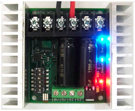
Figure 2: Sabertooth 2x25A V2
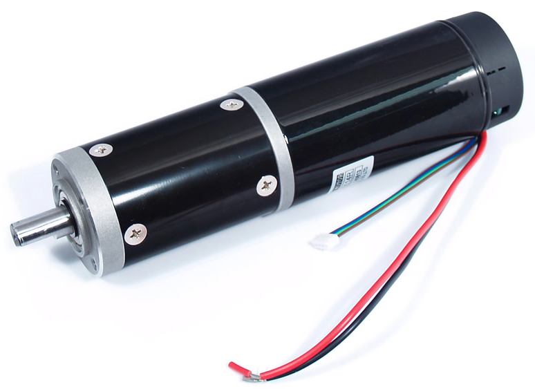
Figure 1: IG52-04 24VDC 285 RPM motor
- Wiring & PCB Design
- Programming the Tiva microcontrollers
- Physical Design & Sensor Placement
- Control of a Single Robot including Odometry Calculation & Verification along with Sensor Fusion
- Formation Control of all Three Robots
Wiring & PCB Design
This section provides a mid-level overview of how all the electronics were connected, starting from the motor and going all the way up to the sensors. Before starting, it should be noted that the motors, motor drivers, chassis, wheels, switches, batteries, gears and chains were all sourced from the Programmable Mecanum Wheel Vectoring Robot - IG52 DB product on SuperDroid Robots' website. As shown in Figure 1, a brushed 24VDC motor, capable of going 285 RPM and complete with a dual channel/quadrature magnetic encoder was used for this project. Four of these were installed in the aluminum chassis with enough combined torque to move the robot while carrying a 200lb payload! In regards to connections, the Sabertooth motor driver (Figure 2) can provide 25A to two motors (one pair of red/black leads wired to M1A/M1B, and the other pair to M2A/M2B). As the motors have a rated current of up to 2.85A, this driver is more than able to do the job. The middle two terminals of the Sabertooth (B+/B-) were then wired to a 24V busbar (powered by two 12V 18Ah Interstate SLA batteries hooked up in series) via a 25A 4PST switch. For safety, a 6.3A Slow fuse was hooked up between B+ and the 24V (2.85A*2 < 6.3A). Since there are four motors, two Sabertooths were installed - one on either side of the robot.
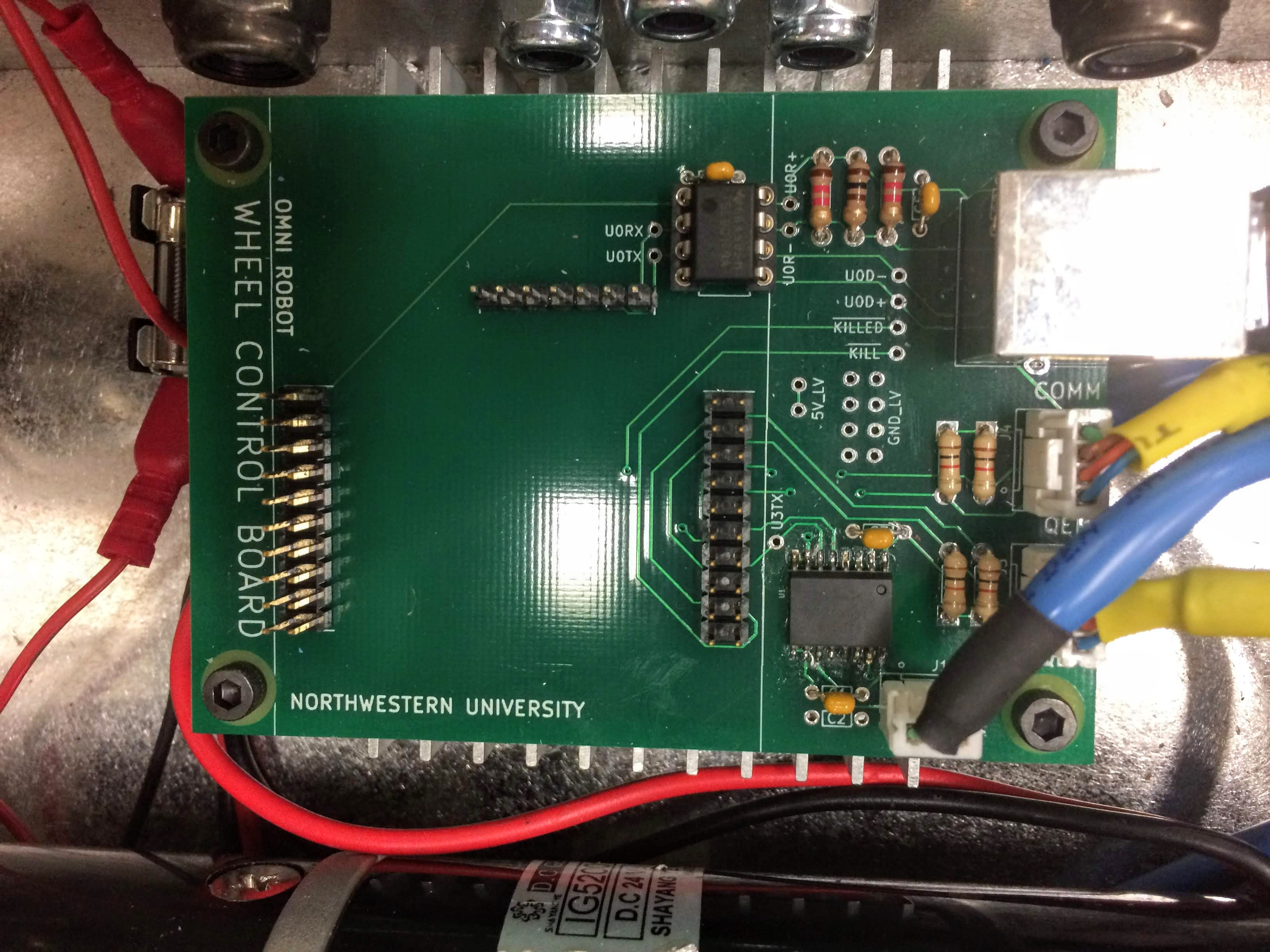
Figure 3: 'Wheel' PCB to control the motors
With a good understanding now of how the motors are powered, the wiring needed to control them can be discussed. In the previous paragraph, I mentioned that each motor has a quadrature encoder which can be used to measure its speed. Four wires come out from the encoder. Two of them represent Channel A and B and the other two provide 5V and Ground. Unfortunately, the Tiva microcontroller that is being used only has two quadrature encoder peripherals (aka QEI pins). As a result, only two motors' encoder wires can be hooked up to any one microcontroller. Thus, two PCBs were made to aid in the motor control process. Known as the 'Wheel Control Board' (shown in Figure 3), each board contains two four-pin JST housings for two sets of encoders (by the yellow heat-shrink in Figure 3). Additionally, it holds a three-pin JST housing (by the black heat-shrink) for three wires that connect to the 0V, 5V, and S1 pins on the Sabertooth (Figure 2). The Tiva microcontroller (which plugs into the header pins on the left half of the board) uses these three pins to send packetized serial commands to the Sabertooth. The 0V pin provides a ground reference for the signal pin (S1), and due to how the packetized serial mode works on the Sabertooth, the Tiva can send commands via the S1 pin to both of the motors hooked up to the Sabertooth. Finally, in order to isolate the 'high voltage' motor driver from the 'low voltage' Tiva board, the ISO3086DWR 16-pin isolated RS485 chip was placed between them. The 'high' 5V from the Sabertooth was then used to power the 'high' side of the chip.
Just as a note, the way to determine where the motor or encoder leads would be attached was based on a 'low' to 'high' number system. Looking in the same direction as the front of the robot, the leads associated with the right side of the robot had a 'lower' number than the left side. For example, the motor leads that powered the right wheel would connect to M1A/M1B on the Sabertooth while the leads that powered the left wheel would connect to M2A/M2B. Similarly, the encoder wires for the right wheel would plug into the QEI0 peripheral while the ones for the left wheel would plug into the QEI1 peripheral.
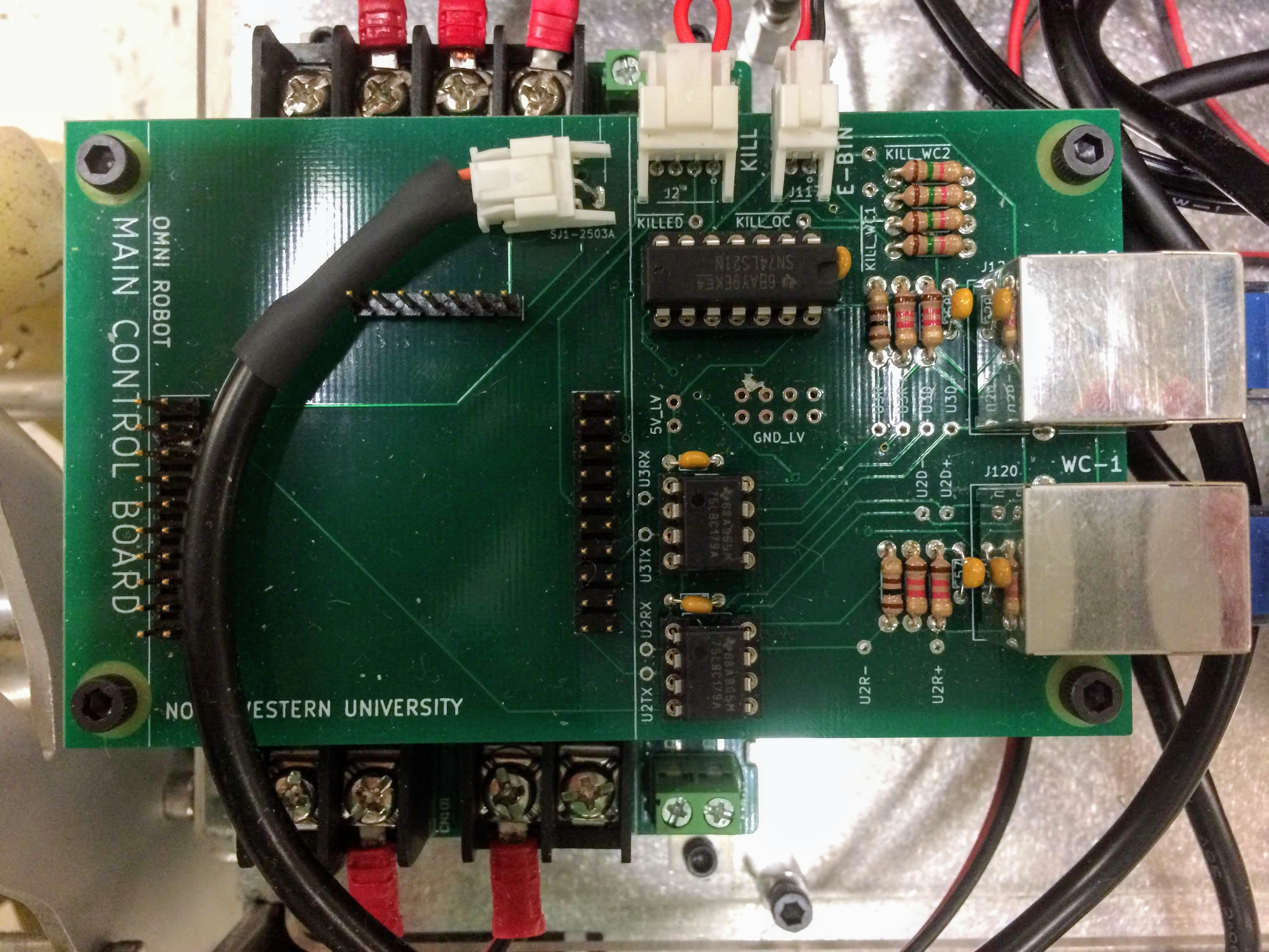
Figure 4: 'Omni' PCB to control the 'Wheel' microcontrollers
Technically, this setup would have been enough to control all four wheels of the robot. An FTDI cable could be hooked up from each Tiva microcontroller (TX, RX, and ground pins) to the NUC (a computer with a 4x4 inch footprint capable of running Ubuntu Linux) and the NUC could send commands through it to both microcontrollers. However, this design idea was discarded for a few reasons: 1) it would require twice the number of USB ports on the NUC 2) there was no guarantee that commands would be sent to each 'Wheel' Tiva at exactly the same time 3) since the Delta robot had a 'master' microcontroller to control the Tivas that directly interfaced with its motors, it would be consistent if the Omni robot had one as well. This is where the Ethernet cables come in handy. As shown in the right part of Figure 4, two Ethernet cables leave the 'Omni' PCB from the two silver rectangular ports. One cable connects to a port on one 'Wheel' PCB (top right in Figure 3) and the other connects to the second 'Wheel PCB'. In order to preserve Serial data, 8-pin RS485 chips (one for each 'Wheel' PCB and two on the 'Omni' PCB) were placed in between the TX and RX pins of the Tiva and the Ethernet port. This accounts for four of the wires inside the 8-wire bundle that make up the Ethernet cable (TX+, TX-, RX+, RX-). Another two wires provide 5V and GND to power the 'Wheel' Tivas. The last two wires were used for Emergency Stop purposes - one for a 'Wheel' Tiva to request an E-STOP (from the 'master' Tiva) and one to get back the response. The 'requests' then become two inputs to an AND gate on the 'Omni' PCB. Another two inputs to the AND gate come from the 'Omni' Tiva itself as well as an external Emergency Stop button (which plugs into the two pin JST in the top of Figure 4). If the Delta robot is being run at the same time as the Omni robot, the output of the AND gate travels up (via the 4-pin JST right next to the two-pin E-STOP JST) to the Delta and becomes an input to another AND gate located on its 'master' PCB. The output from the Delta AND gate (i.e. the 'response') travels back down to the 'Omni' PCB then to the 'Wheel' PCBs. However, if the Delta robot is not connected, the output of the AND gate located on the 'Omni' PCB becomes the 'response' signal (thus, the reason why the 4-pin JST shows a wire looping back on itself - note that the other two pins of that JST do not connect to anything). Finally, the black FTDI cable shown in Figure 4 connects to a USB port in the NUC.
Besides for the 'Omni' FTDI cable, three other micro-USB cables plug into the NUC. One is used to power the 'Omni' Tiva (which then feeds the power to the 'Wheel' Tivas). The other two plug into this laser scanner and this IMU respectively. To power the NUC though is a bigger problem since it only accepts 12-19VDC and because it should be isolated from the 24V motor power supply. To fix this issue, this DC/DC converter was placed between the NUC and the 24V motor power supply (can partially be seen under the 'Omni' PCB in Figure 4). In any event, that about sums up the wiring of the Omni robot!
Programming the Tiva Microcontroller
With an ARM Cortex-M4 core capable of floating point, CPU speeds up to 80 MHz, 256KB Flash memory, 2KB EEPROM, 8 UART modules, 2 Quadrature Encoder Inputs, and a pricetag of only $13.50, the TM4C123G LaunchPad Evaluation Board had everything needed to make this project work. Although in the design from last quarter, the plan was to have each Sabertooth connected to a Kangaroo motion controller which in turn would be wired to a single Arduino Mega, this was rejected for a couple of reasons. For one, the Kangaroo (which would have been responsible for doing PID control to maintain the desired wheel speeds) could not accurately measure the velocity of a given motor. For example, if the Kangaroo was commanded to rotate a motor at 60 rpm, an external tachometer would measure a speed of 55 rpm. A possible explanation for this could be due to the nature of the magnetic encoders on the back of each motor. Normally, Channel A and B should have a 90 degree phase shift between them as shown in Figure 5.
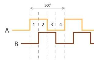
Figure 5: Typical Encoder Trace
However, when measured with an oscilloscope, the traces from the magnetic encoders showed variable phase shifts (ex. if the Channel B trace in Figure 5 was shifted a bit more to the left). Considering the fact that the Kangaroo did give an accurate velocity reading when taking in square wave pulses that were 90 degrees apart (via a function generator), this seems to be the most likely culprit. It is not obvious though why this is the case. Possibly, the Kangaroo calculates speed by measuring time between each quadrature transition. Thus, variable phases between transitions could lead to inaccurate velocity estimates. On the other hand, the Tiva calculates speed by counting the number of quadrature transitions that occur in a specified time frame (20ms in the project). As a result, the variable phase shifts don't matter. Even if the Tiva missed a transition that it would have registerd assuming the channels were 90 degrees apart, it would not make a noticeable difference in the velocity estimate due to the large number of samples already accumulated in that time frame (ex. if the Tiva counted 99 transitions when it should have been 100). For that reason, it was decided to replace the Kangaroos with the Tiva LaunchPads (also because the Delta was using them). Furthermore, it didn't make sense to stick with the Arduino Mega but rather to use another Tiva as the 'master' of the two 'Wheel' Tivas to keep the architecture consistent (and cheaper!).
To actually program the Tiva microcontrollers, the Atom text editor was used in conjunction with the GNU Arm Embedded Toolchain so that programs could be flashed to them. In addition, my advisor (Matthew Elwin) provided libraries containing custom Serial communication protocols and basic peripheral initialization functions that he wrote (originally for the Delta robot) for my partner (Aamir Hussain) and I to use while developing our code. For the first couple weeks of the quarter, we both familiarized ourselves with his code as well as his style of programming so that we could program the microcontrollers for the Omni robot in a similar fashion. Additionally, in order to keep communication between the NUC, microcontrollers, and motors straightforward, it was decided to only allow 'upstream' systems to initiate contact. Specifically, the NUC could send commands down to the 'Omni' Tiva which in turn could send commands down to the 'Wheel' Tivas which in turn could send commands to the motors. However, a 'Wheel' Tiva would not be allowed to send data to the 'Omni' Tiva without first being requested to do so by the 'Omni' Tiva. Likewise, the 'Omni' Tiva would not be able to send data to the NUC without the NUC first requesting it. In any event, after becoming familiar with the microcontrollers, I focused on programming the 'Wheel' Tivas - specifically setting up the QEI peripherals mentioned above, creating a library of functions to interface with the Sabertooths (via packetized serial mode described here), and implementing a PID control loop to set wheel speeds. On the other hand, Aamir focused on programming the 'Omni' Tiva - specifically figuring out how to send Serial commands to both 'Wheel' Tivas at the same time as well as implementing functions to convert wheel velocities into twists and visa versa. This will be discussed more in the next couple paragraphs.
In the process of determining the number of encoder ticks per wheel revolution, the following points were observed.
- There are 19 pulses per encoder wheel revolution.
- Although Superdroid specifies that the gear reduction ratio of the motors is 12:1, it is in fact 12.25:1. Thus, it takes 12.25 encoder wheel revolutions to rotate the motor output shaft just once.
- The gear reduction ratio from the sprocket on the output motor shaft to the sprocket on the wheel axle is 21:15. Thus, for every 21 rotations of the output motor shaft, the actual wheel of the robot rotates 15 times.
- The microcontroller uses x4 encoding so each pulse of the encoder is counted as 4 indivdiual ticks (rising edge of Channel A, rising edge of Channel B, falling edge of Channel A, falling edge of Channel B) which increases resolution by a factor of 4.
Therefore, the number of ticks counted by the QEI peripheral on the Tiva that make up one wheel revolution is: $$ \frac{19\,pulses}{1\,encoder\,wheel\,rev} * \frac{12.25\,encoder\,wheel\,rev}{1\,motor\,rev} * \frac{21\,motor\,rev}{15\,wheel\,rev} * \frac{4\,ticks}{1\,pulse}= \frac{1303.4\,ticks}{1\,wheel\,rev} $$ To convert from ticks/rev to the angular velocity units of rad/sec, the following points were considered.
- The system clock frequency for the Tiva was set to 80 MHz.
- The QEI peripheral has an associated API (found in the TivaWare Peripheral Driver Library here) that allows the user to count the number of encoder ticks per a given period of time (measured in system clock ticks). Currently, this value is set to 1.6 million.
This then leads to the conversion equation below: $$ \frac{x\,ticks}{1.6\,million\,system\,ticks} * \frac{80\,million\,system\,ticks}{1\,sec} * \frac{1\,rev}{1303.4\,ticks} * \frac{2\pi}{1\,rev} = \frac{y\,rad}{sec} $$ Using this equation and PID control, the 'Wheel' Tiva was able to complete its purpose - to get a pair of desired wheel velocities (in rad/sec) from the 'Omni' Tiva, command both motors to achieve those speeds, and send back to the 'Omni' Tiva the current wheel speeds for odometry purposes. Besides for this, the 'Wheel' Tiva was also programmed with functions to change PID values and to save/load them to and from EEPROM.
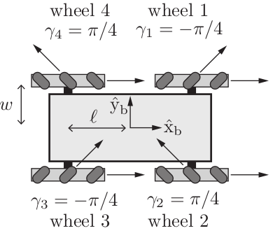
Figure 6: Mecanum Wheel Kinematics (pg. 519 in Modern Robotics)
Once all four wheel velocities are sent to the 'Omni' Tiva, the next step is to calculate the planar twist of the robot. This can be done using Equation 13.33 from Modern Robotics: $$ V_b = Fu \qquad => \qquad \begin{bmatrix} w_{bz} \\ v_{bx} \\ v_{by} \end{bmatrix} = \frac{r}{4} \begin{bmatrix} \frac{-1}{(l+w)} & \frac{1}{(l+w)} & \frac{1}{(l+w)} & \frac{-1}{(l+w)} \\ 1 & 1 & 1 & 1 \\ -1 & 1 & -1 & 1 \end{bmatrix} \begin{bmatrix} u_1 \\ u_2 \\ u_3 \\ u_4 \end{bmatrix} $$ where \(u\) is the vector of wheel velocities (the numbers in the subscript correspond to the ones in Figure 6), \(F\) represents the transformation matrix (\(l\), \(w\), and \(r\) correspond to the measurements shown in Figure 6 and the radius of the wheels), and \(V_b\) symobizes the body twist of the robot. With a little rearranging, the equation above can also convert body twists to wheel velocities as shown in Equation 13.10. $$ u = H(0) V_b \qquad => \qquad \begin{bmatrix} u_1 \\ u_2 \\ u_3 \\ u_4 \\ \end{bmatrix} = \frac{1}{r} \begin{bmatrix} -l-w & 1 & -1 \\l+w & 1 & \;\;\;1 \\l+w & 1 & -1 \\-l-w & 1 & \;\;\;1 \\ \end{bmatrix} \begin{bmatrix} w_{bz} \\ v_{bx} \\ v_{by} \\ \end{bmatrix} $$ where \(H^\dagger(0) = F\). Armed with this equation, the 'Omni' Tiva contains functions allowing the NUC to set a desired twist or get a current twist. By sending the commanded wheel velocities to each 'Wheel' Tiva in a piecemeal manner (switching off sending a few bytes to one, then the other), the 'Omni' Tiva also ensured that both wheels would be set to their new velocities at the exact same time. Furthermore, it should be noted that the 'Wheel' Tiva's control loop operated at 400 Hz while the 'Omni' Tiva's control loop ran at 100 Hz. As such, for those 3 - 4 cycles of the control loop that the 'Wheel' Tiva did not hear from the 'Omni' Tiva, it continued to do PID conrol based on the last wheel velocities that were sent. If for some reason, the 'Wheel' Tiva did not hear from the 'Omni' Tiva for more than 100 of its control loop cycles, it would automatically stop the wheels.
Physical Design & Sensor Placement
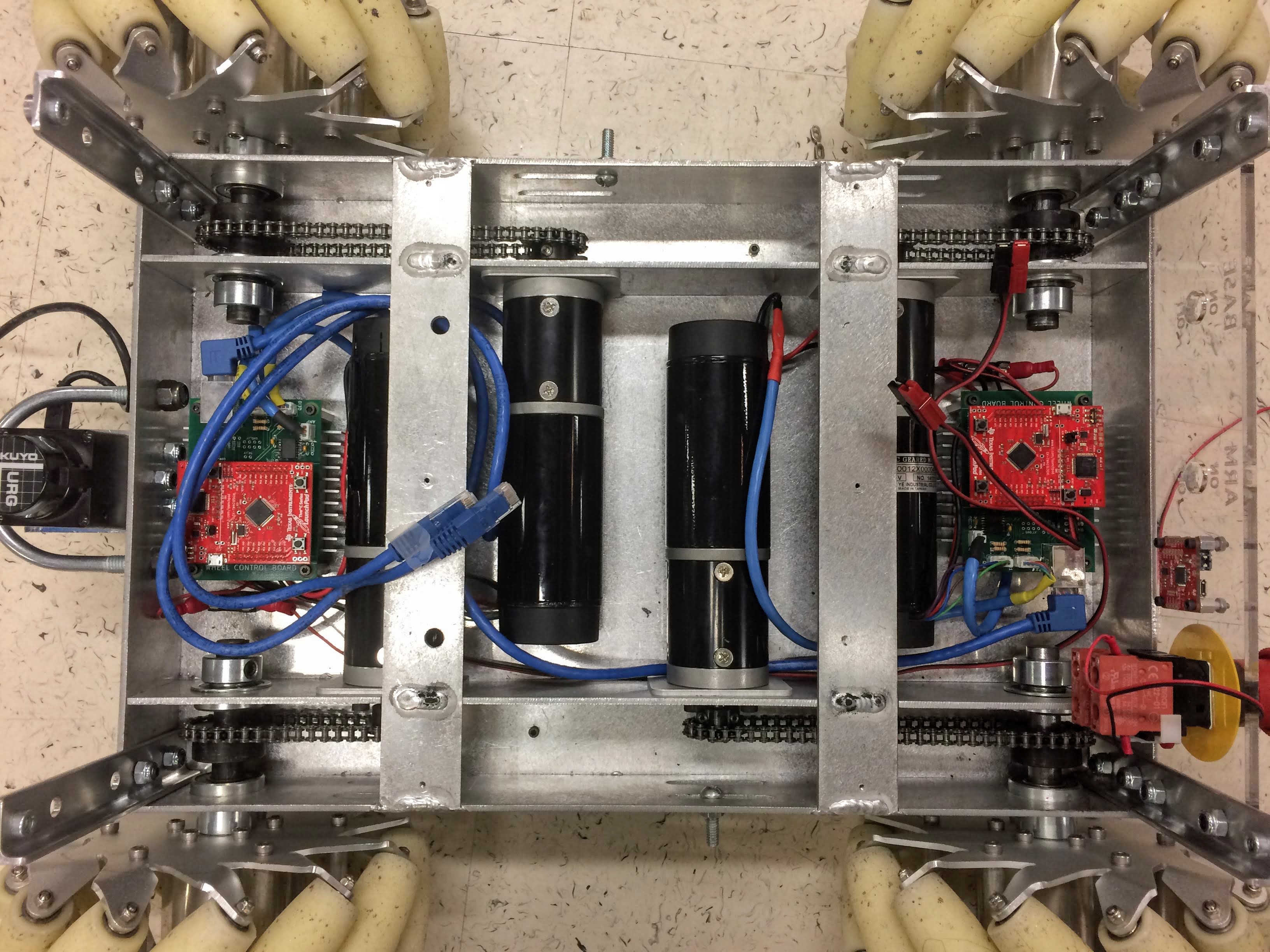
Figure 7: Inside of the Omni Robot
Just like before, I will explain the construction of the Omni robot from the bottom up. After unpackaging, the aluminum chassis already had holes for the ball bearings (2 per axle), upper deck supports (2 per corner), cover (3 evenly spaced per rib), motor output shaft (1 per motor), motor spacer plate (4 per motor), and oval shaped screwdriver holes (2 per motor). In addition to that, 9 additional holes were drilled towards the front and back of the robot to screw down the Sabertooth driver (4 holes), the 'Wheel' PCB (4 holes) and the 6.3A slow fuse (1 hole). To make it easier to drill these holes in the correct spots, a wooden stencil was laser cut with the correct hole placement. Two more holes were drilled on either side of the robot (in the middle) where ESD drag chains were installed to dissipate static (without them, the robot would accumulate static while driving and shock anyone who touched it). Finally, 5 holes were drilled in the front of the robot to accomodate the Hokuyo laser scanner (3 in the middle to hold a 90 degree aluminum bracket and 1 on either side to hold the U-bolt scanner guard). Regarding hardware, only Imperial hex drive steel socket cap screws were used although metric ones were installed on the motor spacer plates (since the holes were made specifically for M5 screws). This decision was made so that the builder would only have to use one type of driver (in this case, a set of Imperial Allen wrenches) and because the Delta robot had the same type of screws. Additionally, it would have been difficult to adjust the motor spacer plate with a conventional (ex. Phillips) screw as the drive chain would have been in the way of the screwdriver. The allen wrench however, could be maneuvered around the drive chain to tighten or loosen a socket screw easily.
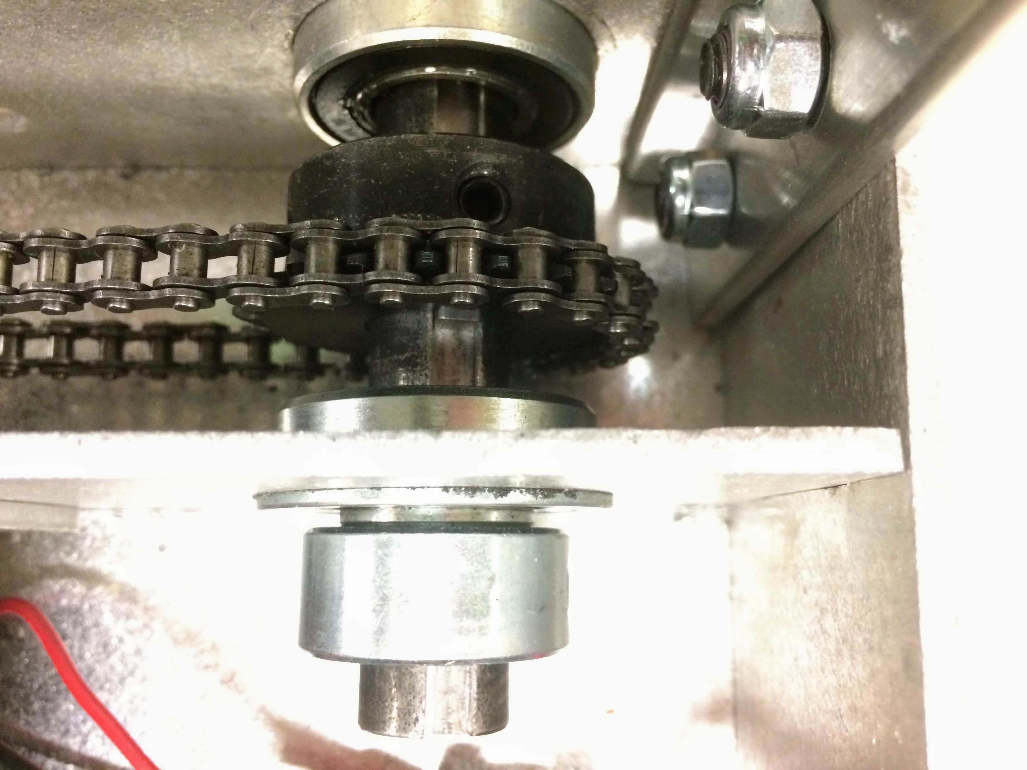
Figure 8: Keyed shaft in wheel axle
To prevent the sprocket on the motor output shaft from slipping, both the shaft and the sprocket were 'D' shaped. Furthermore, all sprockets were installed with set screws that could be tightened to prevent lateral slippage. The sprockets and axle by the wheels however, were keyed as shown in Figure 8. To cut the drive chain to the proper length, a dremmel with a 'grind' top was used, and the procedure outlined in the video at the bottom of this page was followed. In addition, to connect the B+/B- screw terminals on each Sabertooth to 24V, 18 AWG 2 conductor stranded wire was installed with 15A Anderson connectors at the ends. These connectors were then stuck through a small hole in the back of the cover (between the two switches in Figure 9) to click into their counterparts (the red wire leading to the switch and the black wire leading to the GND rail of the busbar). As can be seen in both Figure 9 and 10, another pair of 15A Anderson connectors linked the input of the isolated DC/DC converted (underneath the 'Omni' Tiva) to 24V as well. From a design perspective, the Anderson adapters were chosen due to the easiness of their use, their ability to withstand tremendous current, and to be consistent with the Delta robot where they were also installed. Adding these connectors also helped make the robot more modular. This was especially helpful in the case of the batteries which could be detached from the rest of robot for charging purposes (30A Anderson connectors were used for this purpose).
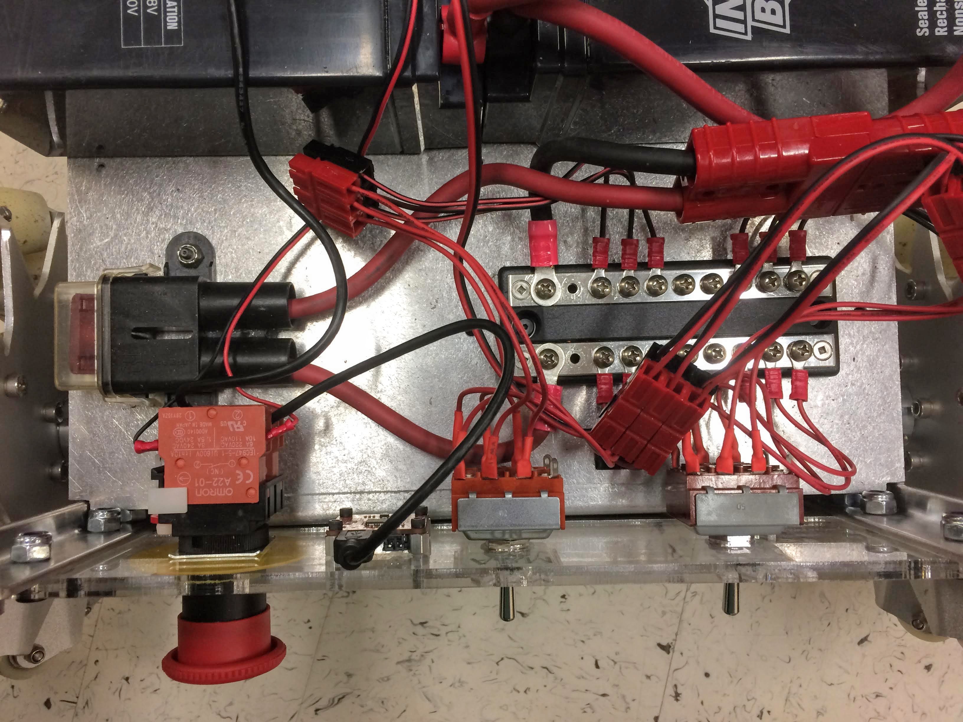
Figure 9: Back of the Omni Robot
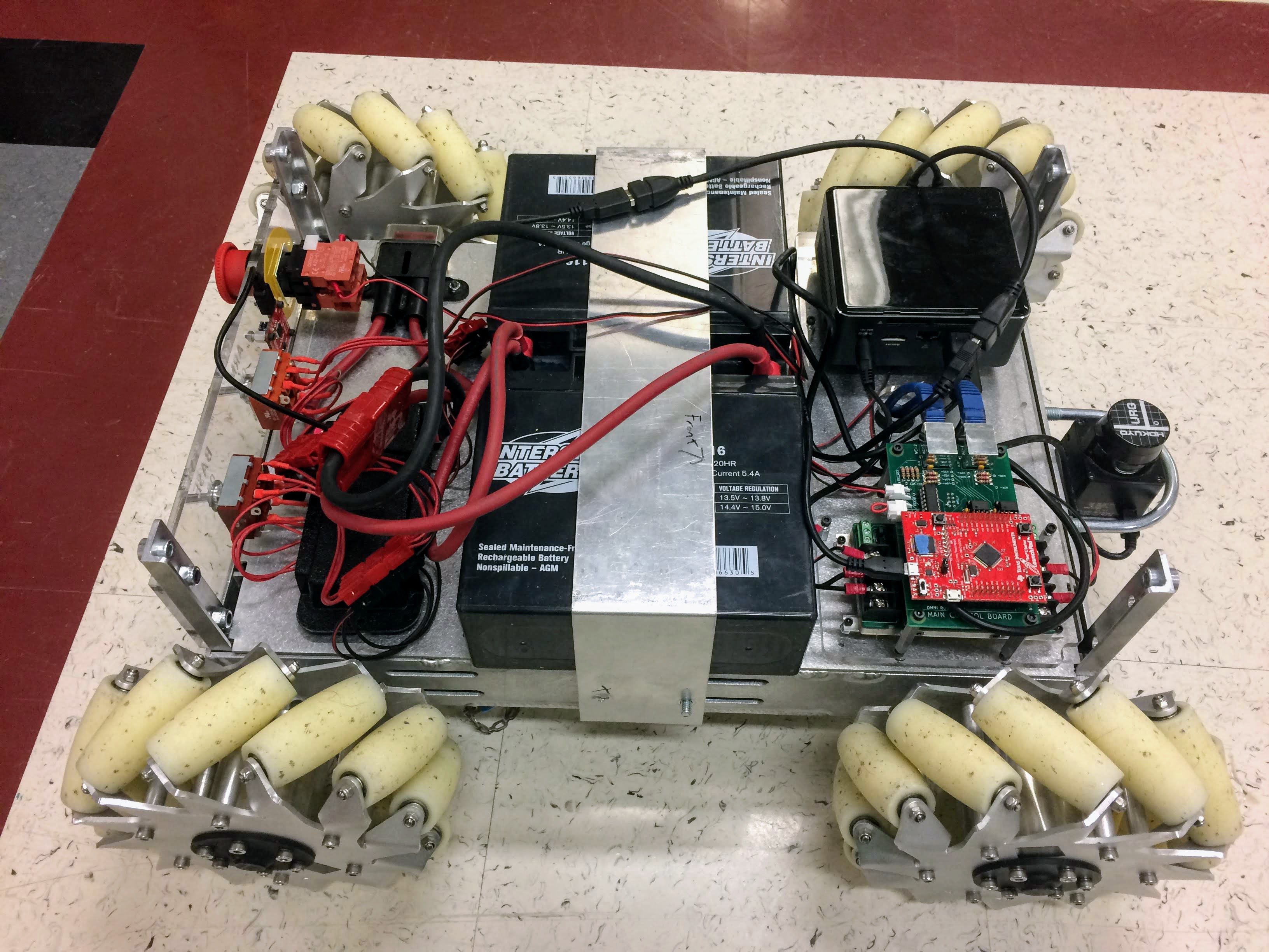
Figure 10: Top of the Omni Robot
Besides for the 6.3A slow fuse by each Sabertooth, there was also a 35A 'system wide' fuse placed between the batteries and the busbar (left part of Figure 9). Additionally, a second switch was placed on the back panel of the robot to power the Delta arm when it will eventually sit on the Omni's upper deck (the first switch obviously powers the Omni robot itself). Lastly, the big red button on the back panel is the Emergency Stop and the object immediately to its right is the Razor IMU. Originally, the IMU was going to be placed at the front of the robot behind the laser scanner, but the magnetic field created by the NUC distorted its magnetometer readings. Fortunately, there was no disturbance observed at the IMU's current location on the back panel.
Moving to the front of the robot, the black square object in Figure 10 represents the Intel NUC computer. Right next to it is a circular hole that allows for the two Ethernet cables originating from the 'Wheel' PCBs to connect to the 'Omni' PCB. Finally, next to that is the DC/DC converter with the 'Omni' PCB ontop, held in place by standoffs. It should be noted that the NUC, DC/DC converter, and 'Omni' PCB are screwed down to a transparent 1/4 inch thick piece of acrylic. This modular 'front deck' was laser cut with all the holes in the correct places to hold the items mentioned above. In turn, the acrylic piece was fastened to the aluminum cover in four places, two of which went through the front rib shown in Figure 7 (thus, the reason for the two holes shown there). Finally, a bracket was placed ontop of the batteries to prevent them from shifting and the upper deck snugly laid down on the four corner supports.
Single Robot Control
Now that the 'Omni' Tiva is capable of sending and recieving individual twists, it was time to create a ROS node to automate the process (initially, this meant commanding a hard coded twist at 100 Hz). Specifically, the node would be responsible for sending the desired twist to the 'Omni' Tiva, recieve the observed twist from the 'Omni' Tiva, and calculate odometry of the robot. To do that, Equations 13.35, 13.36 and a modified version of 13.33 from Modern Robotics were used. It is important to note though that the equations assume that the wheel speeds remain constant between one observed twist and the next (approximately 10ms in this case). In Equation 13.33, the only change is to multiply the right hand side by \(\Delta t\) so that the body twist \(V_b\) is integrated for the right amount of time giving \(V_b = Fu \Delta t\). Next, the difference in coordinates (\(q_b\)) of the robot's new pose relative to its initial pose (before integration) can be found with Equation 13.35. Assuming that \(w_{bz} = 0\), then the change in pose is straightforward. $$ if \; w_{bz}=0, \qquad \Delta q_b = \begin{bmatrix} \Delta \phi _b \\ \Delta x_b \\ \Delta y_b \\ \end{bmatrix} = \begin{bmatrix} 0 \\ v_{bx} \\ v_{by} \\ \end{bmatrix} $$ However, if \(w_{bz}\) is nonzero, then the integration must also take into account the robot's rotation as it calculates \(\Delta x_b\) and \(\Delta y_b\). $$ if \; w_{bz} \neq 0, \qquad \Delta q_b = \begin{bmatrix} \Delta \phi _b \\ \Delta x_b \\ \Delta y_b \\ \end{bmatrix} = \begin{bmatrix} w_{bz} \\ (v_{bx}\sin w_{bz} + v_{by}(\cos w_{bz} - 1))/w_{bz} \\ (v_{by}\sin w_{bz} + v_{bx}(1-\cos w_{bz}))/w_{bz} \\ \end{bmatrix} $$ At this point, we have calculated the change in pose relative to the robot's initial position before integration. However, even if \(w_{bz}=0\), this change in configuration must be transformed into the world frame {\(s\)} so that it can be added to the current odometry estimate. This can be done as follows. $$ \Delta q = \begin{bmatrix} 1 & 0 & 0 \\ 0 & \cos \phi _k & - \sin \phi _k \\ 0 & \sin \phi _k & \cos \phi _k \\ \end{bmatrix} \Delta q_b $$ where \(\phi _k\) is the previous chassis angle relative to the world frame {\(s\)}. Finally, the new odometry estimate can be computed. $$ q_{k+1} = q_k + \Delta q $$
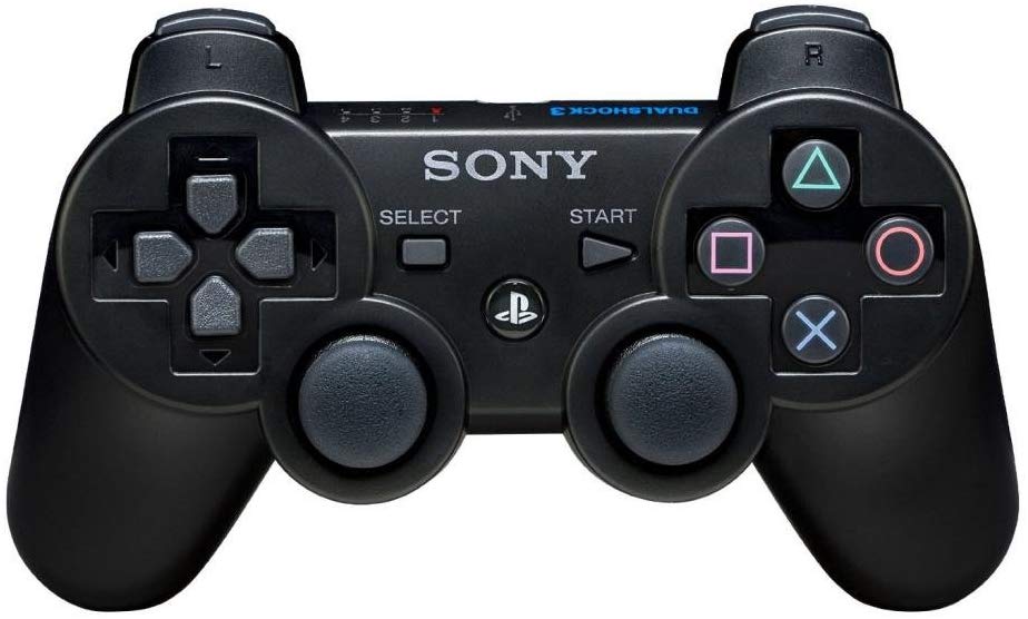
Figure 11: PS3 Controller
With that out of the way, the next step was to send variable twists to the robot. To do that, a Bluetooth enabled PS3 controller (Figure 11) was used. Specifically, the left stick manipulated sideways motion, the right stick manipulated the forward/backward motion and the R2\L2 buttons manipulated clockwise/counterclockwise motion. Besides for this being a logical user interface, another reason these buttons were used was because they were all analog (values ranging from -1 to 1). For this to work with the robot, a new node was created to subscribe to the PS3 messages, stick the correct analog values into a twist message, and send the message to the main node (called 'omni_node') where it would then be commanded to the robot's wheels. While this worked, it sometimes made the robot move in a jerky manner, especially if it was commanded to go from a total standstill to 0.5m/s in one command (or visa versa). To compensate for this, a 'twist filter' was implemented that would allow the robot to slowly build up or decelerate to the desired speed. It would do this by first normalizing the desired twist if one of its values exceeded a velocity limit. Then, it would calculate and send out a new twist based on a user defined acceleration limit. To incorporate this step, the PS3 node would publish a raw twist to the 'raw' filter topic, recieve the updated twist from the 'smooth' filter topic, and then publish the twist (using a custom message as will be explained later) to the 'omni_node'.
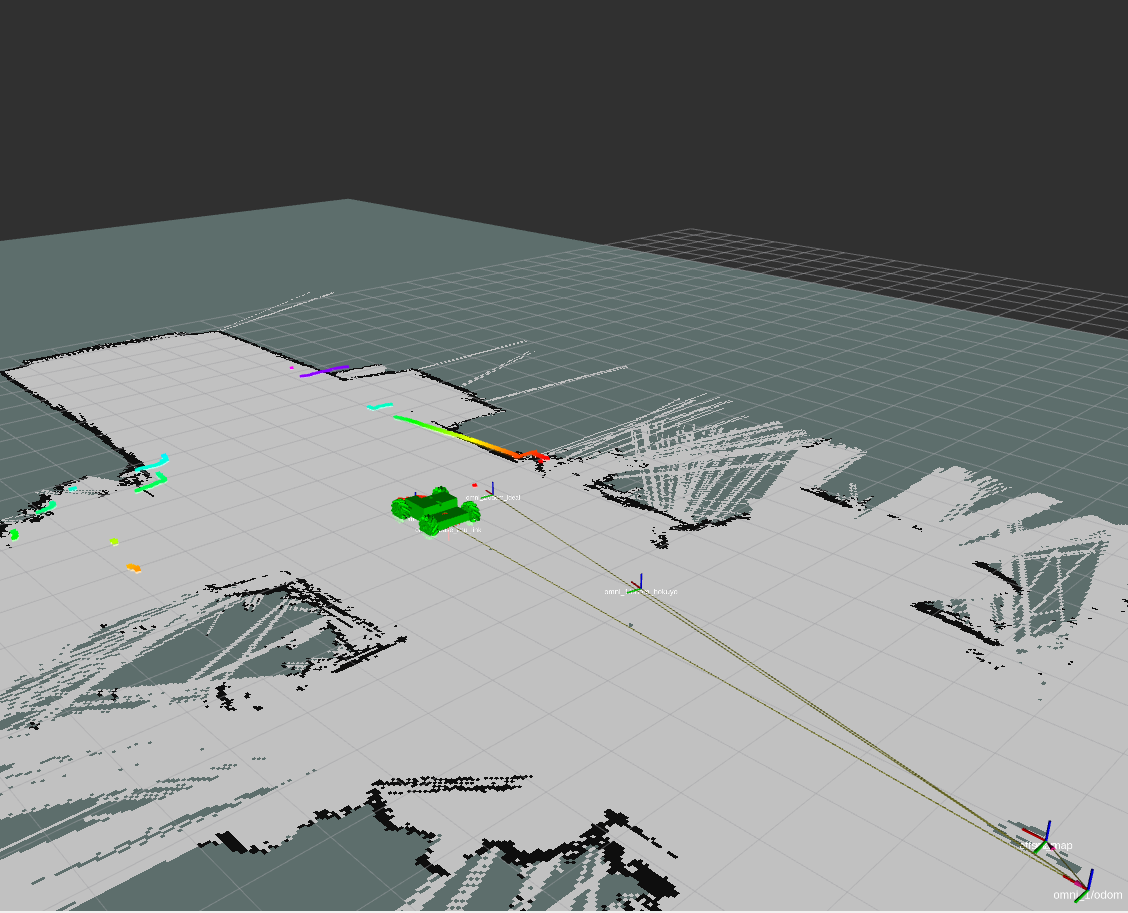
Figure 12: Rviz Demo
Until now, I have been a big vague as to which nodes are run on which computers so as not to confuse the reader. However, this section will clear that up. First, all three robot NUCs are wirelessly connected to a LAN called 'Boeing' (without WAN). A 'master' computer is connected to this network as well although this could be done via Ethernet so that the 'master' retains access to Internet. The responsibilities of the 'master' are to launch the PS3 node (including the twist filter), the Rviz visualization tool (demo shown in Figure 12), and the 'omni client' node (which provides a menu to the user for robot control) on itself. It also is responsible for launching the 'omni node' and sensor related nodes on each of the robot computers (it does this over the network using the 'ssh' tool and preset static IP addresses). Thus, when a user presses a button on the PS3 controller, it is transmitted over Bluetooth to the 'master' computer. After processing the twist via the twist filter, the PS3 node publishes a custom message containing the twist. This is then recieved by each robot's 'omni node' over the network. The custom message specifies an 'id' which tells the 'omni node' which robot should act upon the twist. In this manner, all three robots (or two, or just one) could be controlled with the same twist message. To switch between robot 'ids', the geometrically shaped buttons on the right side of the controller can be toggled.
Regarding odometry verification, there were two methods that were implemented. One method relied on using the 'overhead_mobile_tracker' package developed by Jarvis Schultz. In this case, a camera was placed by the ceiling of the lab and an AR tag was taped onto one of the robots. As the robot moved, the tracker node would publish the tag's odometry which could then be compared with the odometry calculated from the wheel encoders. A python script was developed by Aamir to do just that, and an analysis of the results can be seen on his post. In the second apporach, I compared the odometry of the encoders against those produced by the laser scanner and IMU. This was done by driving the robot an exact distance and comparing the observed odometry values to that distance. A complete write-up of these results including my sensor fusion approach (using the 'robot_localization' package) can be found in the OMNI_SENSOR_SETUP.md file within the 'Boeing' repository. Build and runtime instructions for the Omni robots can be found there as well.
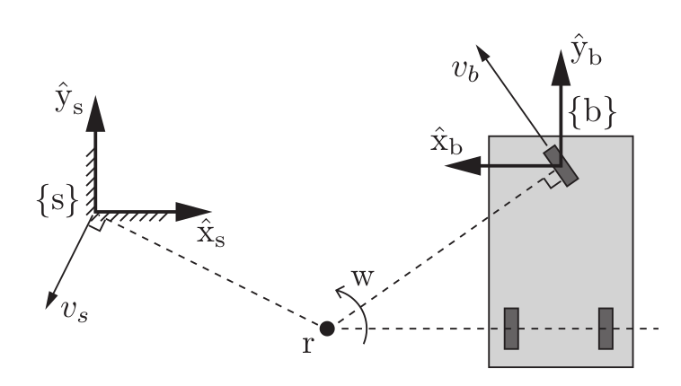
Figure 13: Rigid body motion
Formation Control
The last part of this project was to do formation control of the three robots. Essentially, this means that the user should be able to command a twist to a 'pivot' point, and the robots should move as if they are rigidly attached to that point. To accomplish this, consider the diagram in Figure 13. Ignore the drawn body frame {\(b\)} and assume that \(x_b\) points up and \(y_b\) points left. Also, assume the body frame is at the centroid of the robot as would be the case for a four wheel mecanum wheel robot. Finally, note that \(r\) represents the 'pivot' point. For formation control to work, the following must be given:
- The position of \(r\) in the {\(s\)} frame \(\Rightarrow\) \(r_\theta\), \(r_x\), and \(r_y\). This could be an arbitrary point provided by the user from the 'omni client' menu or the centroid calculated from the robot poses. To be consistent with the picture, we will initialize \(r\) to \([0,2,-1]\) (format of \(\theta\), \(x\), \(y\)).
- The commanded twist \(V_r\) with respect to the 'pivot' frame. This is generated from manipulating the buttons on the PS3 controller. For the sake of this discussion, \(V_r = [\pi/6,0.5,0.25]\).
- The pose of all robots with respect to the {\(s\)} frame. This comes from the odometry calculated for each robot. To fit with the diagram, let's make \(b\) initially \([\pi/2,4,-0.4]\) (format of \(\theta\), \(x\), \(y\)).
In \(V_r\) above, \(w_r = \pi/6\) which means that the pivot is rotating counterclockwise at a rate of \(\pi/6\) rad/s. From this, we can infer that since \(r\) is rotating at \(\pi/6\) rad/s, then any other point on this virtual rigid body is rotating at this angular velocity as well. Thus, \(w_{bz} = \pi/6\), so if this value is not seen in the final body twist, there must be an issue. Moving onwards, we can represent the transformation matrices of the pivot (\(T_{sr}\)) and robot (\(T_{sb}\)) with respect to the {\(s\)} frame as follows: $$ T_{sr} = \begin{bmatrix} 1 & 0 & 0 & 2 \\ 0 & 1 & 0 & -1 \\ 0 & 0 & 1 & 0 \\ 0 & 0 & 0 & 1 \\ \end{bmatrix} \qquad \qquad T_{sb} = \begin{bmatrix} 0 & -1 & 0 & 4 \\ 1 & 0 & 0 & -0.4 \\ 0 & 0 & 1 & 0 \\ 0 & 0 & 0 & 1 \\ \end{bmatrix} $$ Next, we need to find \(T_{br}\), the transformation matrix that represents the pivot frame with respect to the robot. The reason for this will be explained in the next step, but the calculation can be seen below. $$ T_{br} = T^{-1}_{sb} T_{sr} = T_{bs} T_{sr} = \begin{bmatrix} R_{bs}R_{sr} & R_{bs}p_{sr} + p_{bs} \\ 0 & 1 \end{bmatrix} = \begin{bmatrix} 0 & 1 & 0 & -0.6 \\ -1 & 0 & 0 & 2 \\ 0 & 0 & 1 & 0 \\ 0 & 0 & 0 & 1 \\ \end{bmatrix} \qquad and \qquad T^{-1} = \begin{bmatrix} R^T & -R^Tp \\ 0 & 1 \\ \end{bmatrix} $$ where \(p\) represents the 3-vector point and \(R\) symbolizes the rotation matrix. With \(T_{br}\), we can then calculate \(V_b\), the twist in the robot frame, using the Adjoint map (note that \(V_r\) must be padded with zeros to make it a 6-vector). $$ V_b = [Ad_{T_{br}}]V_r \qquad where \qquad Ad_T = \begin{bmatrix} R & 0 \\ [p]R & R \\ \end{bmatrix} \qquad and \qquad [p] = \begin{bmatrix} 0 & -p_3 & p_2 \\ p_3 & 0 & -p_1 \\ -p_2 & p_1 & 0 \\ \end{bmatrix} $$ In the last equation above, \([p]\) represents the skew symmetric form of the point \(p\). When doing the actual calculation for the example above, the result is: $$ V_b = \begin{bmatrix} 0 \\ 0 \\ \pi/6 \\ 1.2972 \\ -0.1858 \\ 0 \\ \end{bmatrix} = \begin{bmatrix} 0 & 1 & 0 & 0 & 0 & 0 \\ -1 & 0 & 0 & 0 & 0 & 0 \\ 0 & 0 & 1 & 0 & 0 & 0 \\ 0 & 0 & 2 & 0 & 1 & 0 \\ 0 & 0 & 0.6 & -1 & 0 & 0 \\ 0.6 & -2 & 0 & 0 & 0 & 1 \\ \end{bmatrix} \begin{bmatrix} 0 \\ 0 \\ \pi/6 \\ 0.5 \\ 0.25 \\ 0 \\ \end{bmatrix} $$
Figure 14: Mathematica Simulation of Formation Control
As was expected, \(w_{bz} = \pi/6\). We also see that the robot is expected to travel 1.2972 m/s along its \(x\)-axis and -0.1858 m\s along its \(y\)-axis. A simulation of this example can be seen in Figure 14. The black arrow represents the space {\(s\)} frame while the green arrow signifies the pivot {\(r\)} frame. Note also that the \(x\)-axis is along the tips of each arrow and the robot markers. Additionally, the red marker marks the location of the robot that we just calculated the twist for. When the GIF resets, one can easily see how the relative location of the arrows and the red marker matches the layout described in Figure 13. The other two markers are there just for show and represent two more robots that have different initial conditions. Most of all, it is readily apparent that all entities move as one rigid body. The reader should note though that the simulation is run at 2x speed.
Demo Video
Credits
This project was the joint effort of four people. My focus was on the following: interfacing with the motor encoders & Sabertooths, designing the 'Wheel' PCB, programming the 'Wheel' Tiva, setting up the sensors, and performing sensor fusion. My partner Aamir Hussain, focused on designing the 'Omni' PCB, programming the 'Omni' Tiva, creating the twist filter, and implementing odometry. Together, we built the physical robots (including wiring, soldering, crimping, drilling, and laser cutting), discussed the theory behind the twist, odometry, and rigid-body-motion calculations, and coded formation control. William Hunt, a staff engineer at Northwestern, took our PCB schematics and created board files using KiCad. Finally, our advisor, Matthew Elwin, helped with all kinds of debugging and provided us with clear goals to follow. An honorary mention also goes to Jarvis Schultz, the Assistant Program Director, who gave time weekly to discuss updates on the project and offer up suggestions.