KUKA youBot Control
Northwestern University: Robotic Manipulation
Technical Skills
- Python
- Rigid-body motion
- Forward & Inverse Kinematics
- Jacobian/Velocity Kinematics
- Trajectory Generation
- Wheeled Mobile Robots/Odometry
- Feedforward, PI Feedback Control
- V-REP robot simulator
Short Summary
In total, this robot has eight degrees of freedom. Five of them are single-axis rotational joints on the arm itself while the other three describe the ability for the chassis to move in the \(x\) and \(y\) directions and rotate in the plane. In the problem, the initial positions of each of these joints are given. To move the end-effector back onto the path, a 5 second control loop was implemented with 0.01 second increments, where at each timestep:
- The current configuration of the end effector, \(X\) was determined using forward kinematics
- The desired configuration, \(X_d(s)\), and twist, \(V_d(s)\) of the end-effector was calculated using the cubic time scaling \(s(t)\).
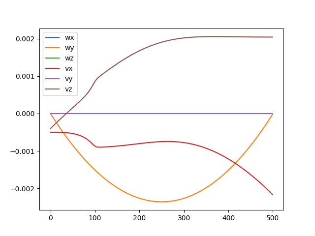
- The error, \(X_{err}\), between the current and desired configurations was calculated.
- The control law below was evaluated to find what the commanded end-effector-frame twist should be. \(Ad\) represents the adjoint of a matrix and is used to change the frame of reference of the feedforward twist \(V_d\) from the desired end-effector configuration, \(X_d\) to the actual configuration, \(X\). $$ V(t) = [Ad_{X^{-1}X_d}]V_d(t) + K_p X_{err}(t)+K_i \int_0^t X_{err}(t)dt $$
- The pseudeoinverse of the combined base and arm Jacobians was then calculated and multiplied by the commanded end_effector-frame twist to obtain the neccessary wheel and joint velocities.
- The configuration at the next time step was simulated using odometry for the chassis and first-order Euler integration for the arm.
At each time step, the configuration was saved to a csv file resulting in a file with 500 rows. The file was then input to the V-REP simulator so that the robot's movement could be visualized. Three different simulations were run with different initial conditions as is explained in the video demo below.
Demo Videos
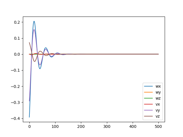
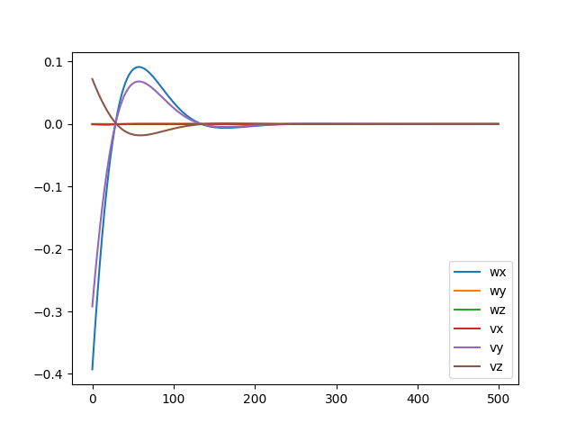
For the case below, the robot started off the path. A proportional gain of 5 and integral gain of 15 were used to bring it back onto the path in approximately 1.5 seconds.
For the case below, the robot started on the path. Only feedforward control was used. Additionally, the error was very small compared to the other cases.
For the case below, the robot started off the path. A proportional gain of 7 and integral gain of 200 were used to bring it back onto the path in approximately 1.1 seconds. As the integral gain was much higher than the proportional one, it was expected that there would be more oscillations.