Inverted Pendulum
Northwestern University: Winter Project
Technical Skills
- ROS
- Python (including Pyserial) & MATLAB
- Robotic Manipulation
- Constrained Inverse Kinematics and Jacobians
- Forward Kinematics
- Microduino CoreUSB, Motion Sensor, and Battery Management Modules
- BlueSmirf Bluetooth Module & Serial Communication
- LQR Control
- Euler-Lagrange Equations with External Forces
- Mathematica Simulation
- Solid Modeling & 3D Printing
Introduction
The objective of this project was to use Sawyer to stably balance a two-degree-of-freedom pendulum. Specifically, the pendulum can only rotate freely along a revolute joint in the 'x-z plane' formed by Sawyer's end-effector (Figure 1). Achieving that goal, the next two goals were to keep the pendulum balancing even with a force disturbance and to balance it at a specific location along the straight line path. To accomplish this, four main tasks were involved:
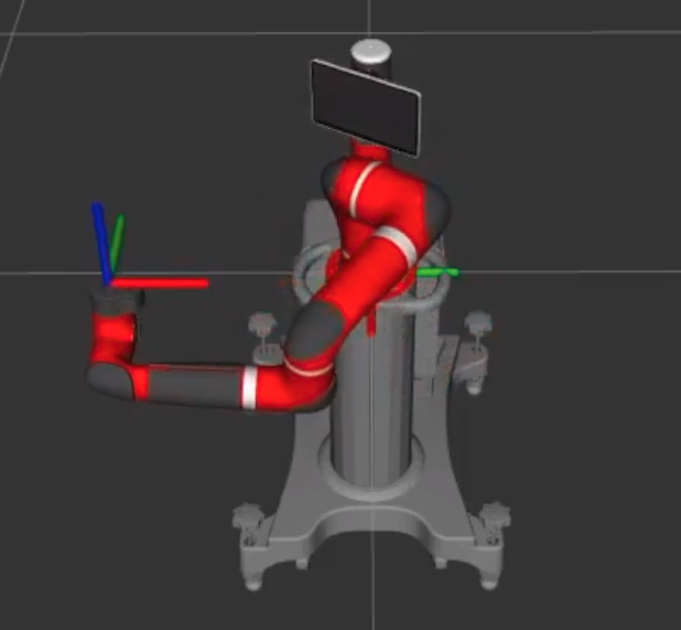
Figure 1: Sawyer's end-effector and base frames
- Calculation of the equations of motion and deriving a Linear Quadratic Regulator (LQR) Controller from them
- Designing a custom inverse kinematics solver to move Sawyer's end-effector along a straight line
- Becoming familiar with the CoreUSB, Motion Sensor, and Battery Management Microduino modules along with the BlueSmirf Bluetooth unit so that angle data could be sent wirelessly from the tip of the pendulum to a laptop
- Solid modeling the attachment to Sawyer's end-effector, the pendulum holder, and the Microduino housing for the top of the pendulum and 3D printing them
I - Part 1: System Dynamics
Assuming a coordinate system where \(x\) corresponds to the position of Sawyer's end-effector (positive is to the right), and \(\theta\) corresponds to the angular position (positive is clockwise) of the pendulum, the equations of motion with an external force, \(F\), are as follows: $$ (m+M)\ddot x + \ddot\theta mL cos \theta - \dot\theta^2 mLsin \theta = F \qquad \Rightarrow \qquad \ddot x = \frac{F+mL(\dot\theta^2\sin\theta-\ddot\theta\cos\theta)}{M+m} $$ $$ \ddot x \cos\theta + \ddot\theta L -g \sin\theta = 0 \qquad \Rightarrow \qquad \ddot\theta = \frac{g\sin\theta-\ddot x \cos\theta}{L} $$ where \(m\) is the mass at the pendulum tip, \(M\) is the mass of Sawyer's end-effector, \(g\) is gravity, and \(L\) is the length of the pendulum. A complete derivation of these equations can be found here. However, the video assumes positive as counterclockwise. Also, the equations here and in the video assume the mass of the pendulum shaft to be negligible and that energy is conserved. A simulation of the inverted pendulum system when \(F = 0\) for some arbitrary values of \(M\),\(m\), and \(L\) can be seen in Figure 2. In all three cases, initial conditions were set to 0 except for \(\theta\) which was set to -0.1 radians or -5.73 degrees.

Figure 2: Simulation of regular equations of motion
Figure 3: Simulation ignoring the dynamics of the 'cart'

Figure 4: Simulation of acceleration control
Figure 2 suggests that with the right feedback, it would be possible to balance the pendulum with an external control force. However, while it is true that Sawyer is equipped with series-elastic actuators that allow forces to be measured (via spring deflections), there are some nonlinearities associated with the measurements that make using force control unreliable. To that effect, I made the decision to work with velocity feedback control. This required a change to the equations of motion. Fortunately, it can be assumed that the motion of the pendulum will have negligible effect on Sawyer's end-effector position. In other words, it can be assumed that if Sawyer's end-effector is commanded to move at a specific rate, it will do so regardless of the pendulum's motion. Thus, the equations of motion can become: $$ \ddot x = u $$ $$ \ddot\theta = \frac{g\sin\theta-u \cos\theta}{L} $$ where \(u\) is the control input. This characterises acceleration control. When the control input is zero, the pendulum is free to swing, but the base (red block in the figures above) does not move (Figure 3). However, with a good control method (look at the section below), \(u\) can be integrated and used as velocity control. It is also interesting to note that the equations above only depend on the length of the pendulum shaft. The longer the shaft, the lower the angular acceleration and the easier it is to control.
I - Part 2: Control Algorithm
To set up the LQR controller, the equations of motion had to first be linearized. To do this, small angle approximation was performed so that \(\sin\theta \approx \theta\) and \(\cos\theta \approx 1\). Thus, the linearized equations of motion are: $$ \ddot x = u $$ $$ \ddot\theta = \frac{g\theta-u}{L} $$ Converting this to state space where the four states are \(x\) - end-effector position, \(\dot x\) - end-effector velocity, \(\theta\) - pendulum tilt, and \(\dot\theta\) - pendulum angular velocity, the following A & B matrices were developed: $$ \dot x = \begin{bmatrix} \dot x \\ \ddot x \\ \dot \theta \\ \ddot \theta \end{bmatrix} = \begin{bmatrix} 0 & 1 & 0 & 0 \\ 0 & 0 & 0 & 0 \\ 0 & 0 & 0 & 1 \\ 0 & 0 & \frac{g}{L} & 0 \\ \end{bmatrix} \begin{bmatrix} x \\ \dot x \\ \theta \\ \dot \theta \\ \end{bmatrix} + \begin{bmatrix} 0 \\ 1 \\ 0 \\ -\frac{1}{L} \end{bmatrix}u $$ After some tuning, the cost matrices for Q and R that gave good results were: $$ Q = \begin{bmatrix} .3 & 0 & 0 & 0 \\ 0 & .001 & 0 & 0 \\ 0 & 0 & 100 & 0 \\ 0 & 0 & 0 & .1 \\ \end{bmatrix} \qquad \qquad \qquad R = \begin{bmatrix} 1 \\ \end{bmatrix} $$ In order to make Sawyer's end-effector movement less aggressive (so that it would be less jerky), I gave small values for \(x\), \(\dot x\), \(\dot \theta\), and \(R\). However, I made \(\theta\) very expensive to 'incentivize' the controller to keep it at 0 degrees. Plugging these matrices into the LQR function in MATLAB, I ended up with following acceleration controller: $$ u = \ddot x = .5477(x-x_{des}) + 1.509\dot x + 30.1922\theta + 8.3422\dot\theta $$ where \(x_{des}\) is the desired position along the straight line path for Sawyer's end-effector. A simulation of this type of control can be seen in Figure 4 where \(x_{des}\) is set to 0.
II Inverse Kinematics Solver
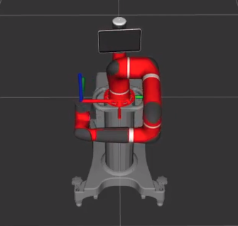
Figure 5: Sawyer's starting position
At program startup, Sawyer's end-effector is placed at the \(SE(3)\) pose shown below (with respect to the base frame) based on some arbitrary joint angles that I thought would be a good starting position. $$ \begin{bmatrix} 0 & -1 & 0 & 0.3447 \\ 1 & 0 & 0 & -0.208 \\ 0 & 0 & 1 & 0.283 \\ 0 & 0 & 0 & 1 \\ \end{bmatrix} $$ To keep the pendulum stable, the end-effector must follow a straight line path parallel to the base frame's 'y-axis' (Figure 5). To achieve this, the transformation matrix above should always be the same except for the \(y\) value (initially -0.208 meters). Well, since I am using velocity control, I should theoretically be able to assign a body twist, \(V_b\), where all velocities are zero except along the 'x' direction (which is equal to the outputted velocity from the controller). Then, using Sawyer's screw axes in the body frame and the current joint angles, the Jacobian can be calculated and used to find the angular velocity at each joint that will move Sawyer's end-effector at the commanded velocity. $$ V_b = \begin{bmatrix} \omega _x \\ \omega _y \\ \omega _z \\ v_x \\ v_y \\ v_z \end{bmatrix} = \begin{bmatrix} 0 \\ 0 \\ 0 \\ v_{control} \\ 0 \\ 0 \end{bmatrix} \qquad \qquad V_b = J_b(\theta) \dot \theta \qquad \Rightarrow \qquad \dot \theta = J_b^ \dagger (\theta) V_b $$ Unfortunately, error starts to build up in the above transformation matrix (specically the \(\omega _x\), \(\omega _y\), \(\omega _z\), \(x\), and \(z\) values) probably becasue real systems are not ideal. As a result, this error between the desired pose and current pose must be rectified. The way I did this was by setting my 'desired' end-effector pose as shown in the transformation matrix above. Then, I calculated the current end-effector pose with forward kinematics using the current joint angles and Sawyer's screw axes (with respect to the body frame) and \(M\) matrix. By taking the inverse of the current end-effector transformation matrix and multiplying it with the 'goal' pose, the 'error' transformation matrix from the end-effector's current pose to the 'goal' pose can be found. This can then be converted into a twist with the matrix logarithm that can be used to keep Sawyer's end-effector from drifting. Finally, the \(v_x\) value in the twist can be thrown out and replaced with the \(v_{control}\) velocity calculated above.
III Hardware
When it came to choosing a microprocessor, I went with the Microduino CoreUSB as it is very small (about a square inch). Similarly, the Microduino Motion Sensor is the same size and stacks right on top of the CoreUSB and contains a MPU6050 IMU. With the Arduino IDE, I modified a version of Jeff Rowberg's code for the MPU6050 (which comes as one of the Microduino example scripts) that uses the onboard Digital Motion Processor to calculate roll angle. I then soldered the BlueSmirf unit to the TX and RX pins on the CoreUSB so that it could transmit the roll angle data wirelessly from the tip of the pendulum (where it would be located) to a laptop. Finally, I stacked Microduino's Battery Management module with the other two and connected it to a 3.7V 110mAh lithium ion battery. All of this was then placed in the solid modeled 'Microduino House' discussed in the 'Solid Modeling' section.
Regarding communication, my original plan was to use ROSSerial. However, this required adding too much overhead which filled up the allowable RAM on the CoreUSB to the point that it became unstable and useless. I then switched to PySerial and created a script in Python to read incoming data from a virtual serial port and publish it to a ROS topic. This worked like a charm and I was soon publishing angle data at a rate of 100Hz.
IV Solid Modeling
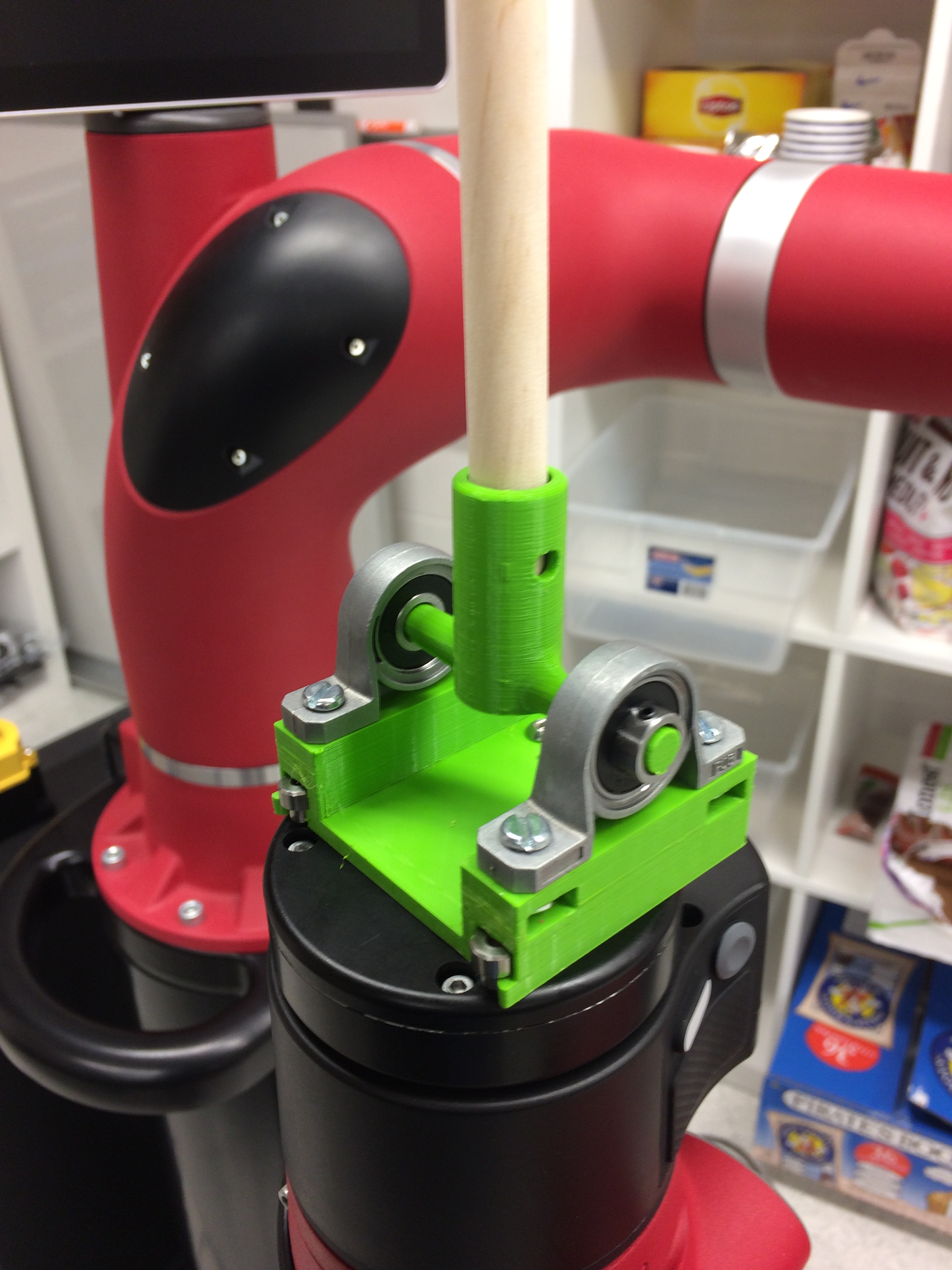
Figure 6: Sawyer Attachment & Pendulum Holder
The three solid modeled parts were designed with OnShape and 3D printed with the help of Cura using the Ultimaker 2 Plus. The 'pendulum holder' was held in place between two pillow-block ball bearings which were screwed down into the 'Sawyer Attachment'. To prevent the holder from shearing in two (which happened in the first trial), it was printed with 100% infill density. Furthermore, screw holes were positioned in the 'pendulum holder' and the 'Microduino House' (not shown) so that the wooden dowel could be kept in place. This was done both to keep the dowel from moving and to align the Motion Sensor module in the 'Microduino House' so that its axes were aligned with Sawyer's base frame axes. Lastly, the top of the 'Microduino House' was cutout in the outline of a sphere so that the wooden ball shown in the demo video could easily rest on top of it. Besides for looking cool, the ball also shifted the center of mass of the pendulum further up (to about 84 cm along the 91 cm shaft), helping with stability.
Demo Analysis
In the video below, Sawyer moves his arm to keep the pendulum from tipping over. In the beginning (until t \(\approx\) 50 sec in the graphs below), it is easy to see how the system remains stable when no external disturbance is taking place (the orange line in Figure 7 is the reference position of -.208 m = \(x_{des}\)). In the second part, the pendulum shaft is pushed with another wooden dowel two times (spikes in the graph at t \(\approx\) 50 sec and t \(\approx\) 75 sec). The first time is a light push which Sawyer is able to recover from pretty well. The second time is a harder push, but Sawyer still manages to recover nicely. Finally, at the end of the video, one can see how the shaft tips over when the control output is turned off (spike in pendulum angle shown in Figure 9 at t \(\approx\) 110 sec).
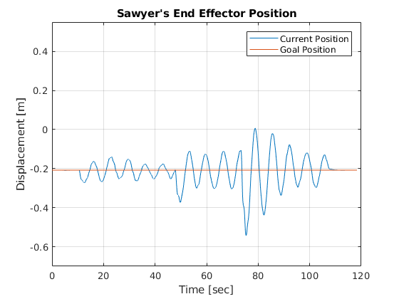
Figure 7: Sawyer's end-effector position
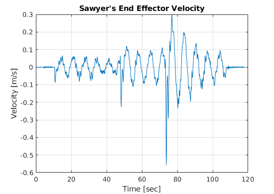
Figure 8: Sawyer's end-effector velocity
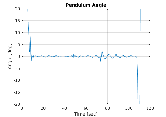
Figure 9: Roll/Tilt angle of the pendulum
To learn more about the project, click here to see the GitHub repo and access the README.