Path Planning With RRT
Northwestern University: Hackathon Challenge
Technical Skills
- Python
- RRT Algorithm
- Minimum Distance between a Point and a Line Algorithm
- Bresenham Line Algorithm
Summary
Three slightly different RRT algorithms were implemented in this project. Before going into them, it is important to first understand how an RRT works. For this explanation, let's assume the world is 100 x 100 and that the robot is at an initial configuration q_init of (50,50). This point is the root of the RRT tree. The algorithm begins when a random point (aka vertex) is generated. Next, the algorithm checks to see what the Euclidean distance is from every vertex in the tree (right now, that's just (50, 50)) to that point. Assuming the distance is less than or equal to delta_q, a line is drawn between the two points. However, if the distance is greater than delta_q, then only a line that is delta_q in length is drawn from the nearest vertex in the direction of the randomly generated point. Finally, this process repeats until the specified number of vertices is added to the tree.
Figure 1: Simple RRT Exploring
RRT Exploring
Figure 1 shows an animation of the RRT process. In this example, q_init = (50,50) and the map size (aka world) is 100x100. Additionally, there are 200 vertices and delta_q = 7. For those cases where the distance between the generated point and the nearest vertex is greater than delta_q, the point along that line that is exactly delta_q away is found using the formulas below. $$ (x_1, y_1) - (x_0, y_0) = (v_1, v_2) = \mathbf v \qquad \qquad (1)$$ $$ \mathbf u = \frac{v}{||v||} = (\frac{v_1}{\sqrt{v_1^2 + v_2^2}}, \frac{v_2}{\sqrt{v_1^2 + v_2^2}}) \qquad (2) $$ In Equation 1 above, \((x_1, y_1)\) represents the randomly generated point while \((x_0, y_0)\) represents the nearest vertex in the tree. \(\mathbf v\) represents the unnormalized vector. In Equation 2, \(\mathbf u\) represents the normalized unit vector that can then be multiplied by delta_q to get the desired point.
Figure 2: RRT With Analytical Collision Detection
RRT With Analytical Collision Detection
In this scenario, the algorithm is not allowed to draw lines if they would pass through one of the black circular obstacles. To determine if this is the case, the minimum distance between the center of every circle and the candidate line can be found. If the distance is greater than the radius of the circle, then the line was drawn. In general, the minimum distance between a point and a line is when a line drawn through the point intersects the original line at a perpendicular angle. However, this is not foolproof as it is possible for this intersection to take place outside the boundaries of the line segment. In this case, the minimum distance is between the center of the circle and q_new (i.e. one of the two points that defines the line segment and is not yet in the RRT tree). Two methods were implemented to find the minimum distance. One is based on this page which does not give a very detailed explanation of how the algorithm was derived. For that reason, I developed a second method based on this video. As shown in Figure 2, the green dot represents the root of the tree while the red dot represents the target. Once the RRT algorithm discovers a vertex that is in clear sight of the target (no obstacles in the path), a line is drawn, even if the line is more than delta_q in length. Finally, the path from the root to the target is highlighted in orange.
Figure 3: RRT With Pixel-based Collision Detection
RRT With Pixel-based Collision Detection
Similar to the scenario above, this third and final algorithm is not allowed to draw lines if they would pass through any of the purple colored pixels. However, unlike the last scenario, there is no way to play off the geometry of the obstacles to determine if a candidate line is in collision. This is where the Bresenham Line Algorithm comes in handy. As we know, it is easy to draw a line between two points on a piece of paper. However, this is not the case on a monitor screen which has a limited number of pixels. The question one must answer is which pixel should be filled in to best represent the line? For example, should it be the pixel in the same row as the first but in the neighboring column? Or, should it be the pixel in the row below and the neighboring column? On a high level, the Bresenham algorithm answers this question by comparing the distance from the theoretical line to the nearest pixel above and below it. Then it fills in the pixel that is closest to that line. Additionally, the algorithm only uses integers in its computation to make the process more efficient. Thus, to determine if a candidate line passes through an obstacle, the Bresenham algorithm is used to check the pixels in the image that would've been used to create the line. Assuming none of the pixels are colored, the line is then drawn. However, this is not 100% foolproof as shown in the images below.
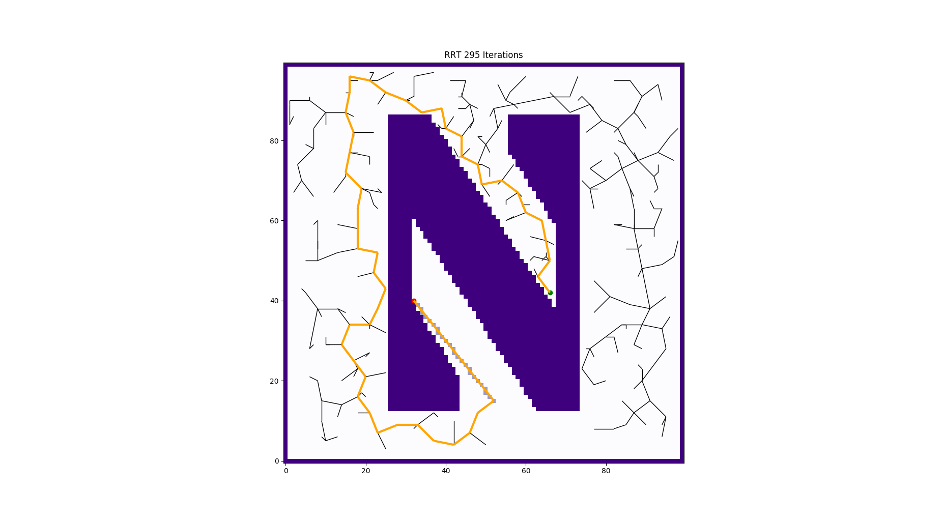
Figure 4: Bresenham algorithm builds a line of pixels from the target to the nearest vertex (light purple shade)
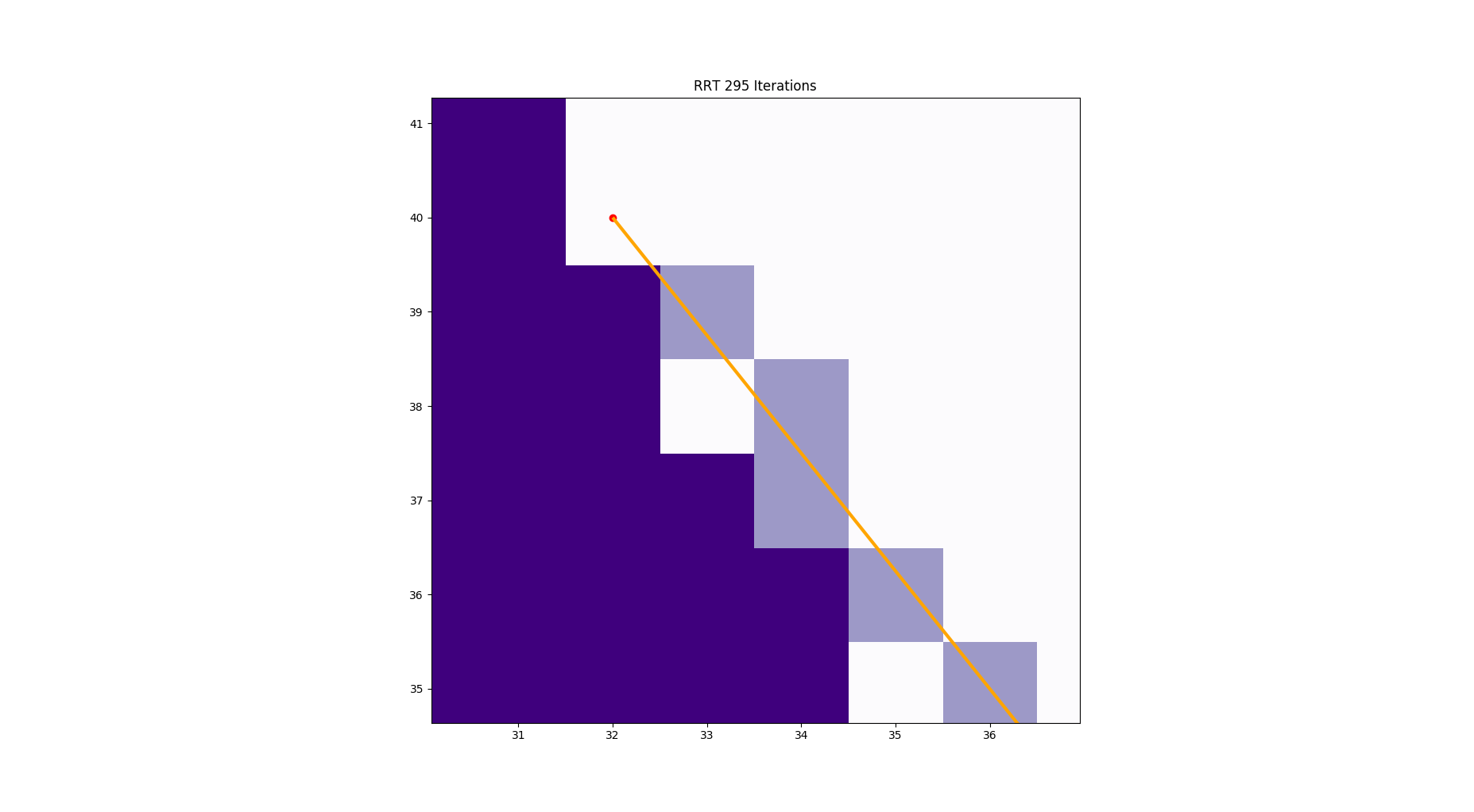
Figure 5: Close up of the line of pixels drawn by the Bresenham algorithm (light purple shade)
It is apparent from Figure 5 that the pixels that make up the Bresenham line (light purple color) do not overlap the deep purple ones. As such, this would imply that the path is obstacle free. After a closer look though, one can see that the orange line does indeed overlap the top right corner of the deep purple pixel located at (32, 39). This could be remedied by checking pixels around the one chosen by the algorithm, but this would take more time and is beyond the scope of the project. For further reference, check out this link which includes some pseudocode that was implemented in this project. Also, look at the video here that does a great job explaining the derivation of the formulas as well as the video here which goes through an example.