DC Motor Control
Northwestern University: Introduction to Mechatronics
Technical Skills
- C Programming Language
- Interrupts & Timers
- Digital I/O pins, PWM via Output Compare
- Analog to Digital Converter
- PIC32MX795F512H microcontroller
- Brushed DC Motor control with H-bridge, encoder, and currrent sensing chip
- PID Controller Design
- Motion Control
- Serial Communication between the PIC and MATLAB
- Circuit Design including low-pass filters & non-inverting gain amplifiers
Short Summary
The goal of the final project in this class was to have a motor follow a reference trajectory accurately. To do this, the block diagram shown in Figure 1 was implemented.
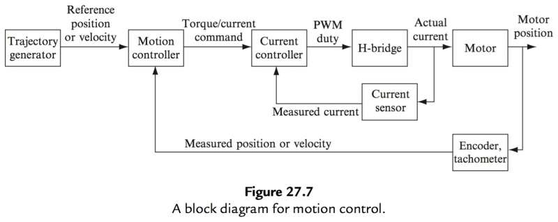
Figure 1: Motion control block diagram (taken from the class textbook, here)
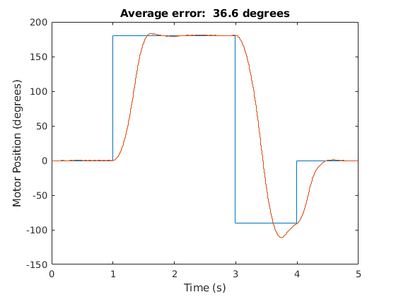
Figure 2: Step Reference & Actual Trajectories
In the beginning of the process (Trajectory generator), a user inputs their desired motor positions into MATLAB. For the step trajectory in the demo video below, this was $$ [0, 0; 1, 180; 3, -90; 4, 0; 5, 0] $$ In other words, at time 0 seconds, the motor angle should be 0 degrees; at time 1 second, the motor angle should be 180 degrees, etc. This can also be seen graphically by the blue line in Figure 2. MATLAB then sends the trajectory over to the PIC microcontroller using UART.
The Motion Controller then reads the current motor position from the Encoder (over SPI) and subtracts that from the reference angle to get the error. It does this in an interrupt that uses a timer to call it at 200 Hz. A PID controller takes the error and outputs a reference current that the current going throught the motor should track to stay on target. After some tuning, the gains that gave the best results were found to be \(K_p = 60.5\), \(K_i = 0\), and \(K_d = 1700\).
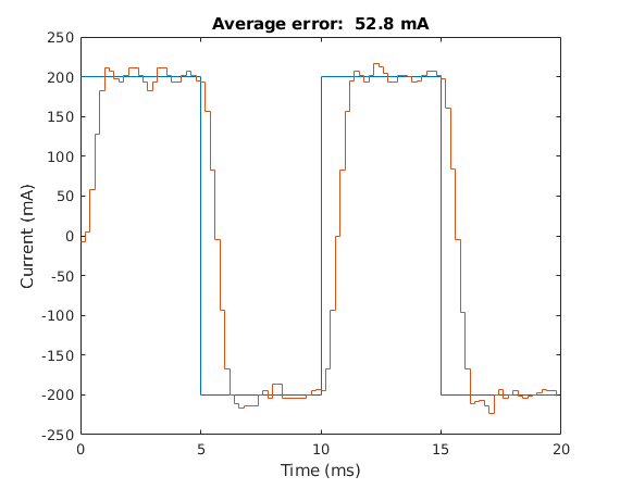
Figure 3: Testing current gains
Similarly, the Current Controller reads the current current from a Current sensor and subtracts that from the reference current to get the error. The current sensor works by measuring the voltage drop across a 15\(m\Omega\) resistor. This voltage is then amplified so it can be easily read on an analogue input pin on the PIC. With a 'calibration' equation, an estimate of the current can be calculated from the ADC reading. As before, this process occurs in an interrupt that uses a timer to call it at 5 kHz. A PID controller takes the error and outputs a duty cycle that changes the average voltage across the motor (and thus current through the motor), so that the requested trajectory can be followed. After some tuning (where success was measured by how well motor current tracked a 100 Hz \(\pm\)200mA reference current square wave - Figure 3), the gains that gave the best results were found to be \(K_p = 0.8\), \(K_i = 0.5\), and \(K_d = 1\).
To set the PWM frequency controlling the supply of voltage across the Motor (via an H-bridge), a timer was used to generate a 20 kHz signal on an Output Compare pin. Then, as mentioned above, the duty cycle was adjusted to track the reference current.
Demo Analysis
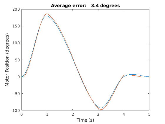
Figure 4: Cubic Reference & Actual Trajectories
In the demo video below, the current gains for the current PID controller are shown followed by a \(\pm\)200mA reference current square wave test to show how well they worked. In this case, the average error was 53.6 mA which is pretty good for a step reference. Next, the step trajectory shown above is inputted into MATLAB and executed. The graph is then shown (orange corresponds to the actual trajectory) where the average error is found to be 36.9 degrees. Again, this is pretty reasonable for a step input of this type. Then, a cubic trajectory with the same times and angle values as for the step trajectory are inputted. The two types are different in that the cubic reference trajecotry gradually changes from one commanded angle to the next (Figure 4) whereas the step trajectory instantaneously jumps from one commanded angle to the next. The trajectory is then executed and another graph is shown. This time, the error was 3.5 degrees which is pretty good. Finally, the Motion Controller PID gains are changed to random values to show the effect of bad gains for both the step and cubic reference trajectories.